Fundamentals of Vibration Control

Laboratories and industrial facilities contain a variety of vibration sensitive equipment used for research and production in fields such as laser-based research, high-resolution imaging, semiconductor manufacturing, and biotechnology. Inserting electrical probes into nuclei of living cells, etching sub-micron lines in nanostructures, or taking SEM images requires laboratory environments to have vibration levels well below human perception thresholds. Floor vibrations can cause imaging components, specimens, lasers, or substrates to move relative to each other, causing blurry images, low yields, and erroneous results. The degree to which this relative motion affects results depends on the amplitude and frequency of the environmental vibrations as well as the sensitivity of the experiment. Common sources of noise and vibration are shown in Figure 1.

Vibration control systems that include vibration isolators and optical tables, are intended to minimize the impact of environmental vibration. The optical table serves as a common base for the whole opto-mechanical assembly. Opto-mechanical components such as posts, rods, and mounts, as well as positioning stages, are made to anchor optical elements in place so that the optical paths will be undisturbed by environmental impacts such as vibration. This section describes the fundamentals of vibration and how these concepts relate to measurable parameters such as compliance and maximum relative motion. These concepts are then used to understand how various systems implement isolation and damping to minimize the impacts of vibration.

Vibration is essentially a periodic force. In order to understand its potential impact on an optical component, it is instructive to start with a simple model that assumes a rigid body (the optical table to which the component is attached) is coupled via a spring to an applied force (the vibration). The resulting interaction can provide a lot of information about how the body moves in response to the force, including the magnitude of the movement and its frequency response. Introducing a mechanism that allows for this movement to be deadened or reduced, i.e., damping, provides for a more realistic system. While this damped harmonic oscillator model is instructive, real structures, such as an optical table, are much more complicated since they can undergo complex deformations when they experience vibrations. The compliance of a system describes how such a structure moves as a result of an external force. While this parameter is both descriptive and quantitative, other parameters such as the relative motion can provide more germane information about how an optical component attached to a table will respond to vibration. These concepts describing responses to vibration are detailed below. Vibration and vibration isolation are both intimately connected with the phenomenon of resonance and simple harmonic motion. One example of harmonic motion is a mass connected to a flexible cantilevered beam (see Figure 2). An external force, either from a one-time impulse or from a periodic force such as vibration, will cause the system to resonate as the spring alternately stores and imparts energy to the moving mass. The frequency at which the system resonates is called the natural frequency. In the example of the mass and beam, the natural frequency is determined by two factors: the amount of mass, and the stiffness of the beam, which acts as a spring. As illustrated in Figure 2, a lower mass and/or a stiffer beam increase the natural frequency while a higher mass and/or a more compliant (softer) beam lower the natural frequency. This example represents an undamped system in which there is no mechanism to dissipate mechanical energy. With a small amount of damping, the system will vibrate for quite a long period of time before coming to rest. Damping dissipates mechanical energy from the system and attenuates vibrations more quickly. For example, when a finger touches the resonating mass-beam system lightly, this damping action rapidly dissipates the vibrational energy.

More formally, as shown in Figure 3, the simple harmonic oscillator consists of a rigid mass M connected to an ideal linear spring. The spring has a static compliance C, such that the change in length of the spring (Δx) that occurs in response to a force F is: Δx = CF. The compliance of the spring is its susceptibility to move and is the inverse of the spring stiffness (k). When the system oscillates, its natural frequency (ω₀) is given by: ω₀ = √1/CM

The natural frequency of the system is determined solely by the mass and the spring compliance. It decreases for a larger mass or a more compliant (softer) spring. The ability to control this resonance frequency is critical in the proper design of optical tables when the goal is to reduce the impact of vibrations (see Vibration Control Systems). If the spring-mass system is driven by a sinusoidal displacement, e.g., vibration, with frequency . and peak amplitude |u|, it will produce a sinusoidal displacement of the mass M with peak amplitude |x|. The steady-state ratio of the amplitude of the mass motion |x| to the spring end motion |u| is called the transmissibility T. This transmissibility is a function of the driving frequency . as shown in Figure 3. There are three key features of this system. Well below the resonance frequency (ω << ω₀), T = 1 and so the motion of the mass is the same as the motion at the other end of the spring. Near resonance (ω ≈ ω₀), the motion of the spring end is amplified, and the motion of the mass |x| is greater than that of |u|. Above resonance (ω >> ω₀), the displacement |x| decreases in proportion to 1/ω². In this case, the displacement |u| applied to the system is not transmitted to the mass. The spring acts as an isolator. Controlling the transmissibility curve is the key to designing effective isolators as shown in Vibration Control Systems.

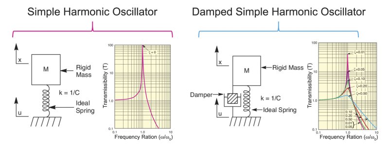
A more realistic system includes a mechanism to dissipate mechanical energy from the system (very often as heat). A damped simple harmonic oscillator is shown schematically in Figure 3. A rigidly connected damper is expressed mathematically by adding a damping term proportional to the velocity of the mass to the differential equation describing the motion. Similar to the undamped system, an external force results in a displacement amplitude of the spring, which is related to the mass displacement by the transmissibility. Plots of T versus ω are shown in Figure 3 for various values of the damping coefficient (ξ). When ξ approaches zero, the curve becomes exactly the same as for the undamped system. However, as the damping increases, the amplitude at resonance decreases and the "roll-off" at higher frequencies decreases, i.e., the transmissibility declines more slowly as damping increases. It is the reduction in amplitude at resonance that explains why the use of damping is a key strategy in both the design of optical tables as well as isolators (see Vibration Control Systems). 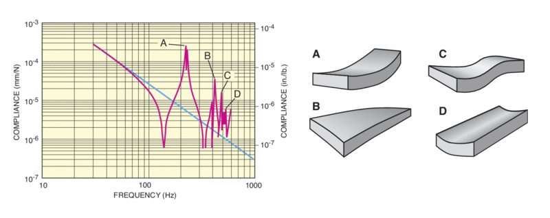While the discussion of a rigidly connected mass-spring system is informative, no actual structure is a perfectly rigid body. All structures vibrate by flexing and twisting. The response of structures to random vibrations can be quite complicated because they vibrate with complex deformations and have more than one resonant frequency. The resonant frequencies of an object are the natural frequencies of vibration determined by the physical parameters of the vibrating object. The compliance curve, the classic method of measuring dynamic rigidity, is a useful tool for evaluating the basic dynamics of a vibrating structure. Compliance is a measure of the susceptibility of a structure to move as a result of an external force. The greater the compliance, i.e., the lower the stiffness, the more easily the structure moves as a result of an applied force, e.g., vibration. Compliance curves show the displacement amplitude of a point on a body per unit force applied (C = |x| / |F|), as a function of frequency. The units of compliance are typically given in mm/N or in/lb. The dynamic performance of a table top is usually characterized with a compliance curve, a log-log plot of the table's dynamic response to random vibration (see Figure 4). The compliance of a rigid body is proportional to 1/ω² and is graphed as a straight line with slope of -2. This line, which is called the ideal rigid body (IRB) line, represents the dynamic performance of a theoretically perfect rigid table. For non-rigid bodies, a compliance curve shows the structure's resonant frequencies and its maximum amplification at resonance.

Figure 4 shows the relationship between an undamped table top's vibration modes and the peaks on its compliance curve. Each peak in the curve, marked A through D, corresponds to a fundamental vibration mode. A table top's response to vibration depends on the frequency range. For low frequencies, the compliance decreases inversely proportional to ω². In other words, the structure is behaving as an ideal rigid body. For frequencies greater than 80 Hz, the compliance curve begins to deviate from this line, structural vibrational modes are excited, and the table begins to deform. The rigid body compliance falls off rapidly as frequency increases, so the largest displacements are generally caused by low-frequency resonances. The first peak on the left (~ 220 Hz in Figure 4) usually has the highest amplitude and dominates the table's response to vibration. The highest possible minimum resonant frequency is desirable, because the amplitude of table displacements is much smaller at higher frequencies, providing greater stability. Damping of table top resonance modes is critical for maximum stability. Effective table top damping reduces compliance, i.e., reduces the height of resonance peaks. The goal is to design a table top whose compliance curve deviates as little as possible from its theoretical IRB line. With other information, compliance curves can also furnish a reliable estimate of how a particular system will perform in a particular application. Maximum amplification at resonance, or Q, is a measure of how much the compliance curve deviates from the IRB line. In exact terms, it is defined as the maximum compliance value of the highest peak above the IRB line (usually, but not always, the first peak on the left) divided by the IRB response at the same frequency (see Figure 5). The lower the Q a structure has, the better it is damped and the more stable the structure will be. A structure that is more stable is less likely to vibrate in response to disturbances. The compliance curve supplies information on the two key parameters that govern dynamic performance Ñ minimum resonant frequency and maximum amplification at resonance. These values can be used to calculate more meaningful table top specifications such as the dynamic deflection coefficient and relative motion. The dynamic rigidity of a table top, i.e., the resistance of the top surface to movement to vibration, is the single most important measure of vibration control performance. But compliance curves, the classic method of measuring dynamic rigidity, do not go far enough in providing a quantitative measure of table top vibration control capabilities. The dynamic deflection coefficient, a figure of merit that can be derived from any compliance curve, enables one to compare dynamic performance directly. When the ambient vibration level is known, the dynamic deflection coefficient can be used to calculate the relative motion value, which can then be used in selecting the most appropriate table for an application. The equation for the maximum relative motion is shown in Figure 5. This equation allows for calculation of the worst-case relative motion between two points on a table at the natural frequency (f_n). Each term can be understood in terms of the physical mechanisms described in the previous two sections. The dynamic deflection coefficient (second term in the equation) is derived from the table top's minimum resonant frequency and damping efficiency, which together quantify the table top's dynamic performance. The third term, the applied power spectral density (PSD), is the contribution of the applied vibration intensity level, which can be measured directly or estimated using a table of typical values. Isolator transmissibility, the fourth term, accounts for the attenuation of ground vibrations at the frequency range of interest through the support structure. Values of the dynamic deflection coefficient and relative motion for a typical lab environment are often specified for an optical table.

One important practical example of using the maximum relative motion is to approximate worst-case beam deflection. The simple setup illustrated in Figure 6 (a mirror mount attached to a table top) indicates how a laser beam reflected by the mirror will be affected by two types of vibrational modes: axial deflection from translational table top motion and angular deflection caused by table top bending motion. Essentially, displacement in translation does not cause significant deflection in most experiments or applications. However, table top bending can have serious consequences for optical performance for two reasons: when a mirror is rotated, the angle of the reflected beam is twice the tilt angle and the "doubled" error also increases linearly with reflected spot distance from the mirror. This effect, multiplied by the number of mirrors in an optical system and the total path length, can have a significant effect on experimental results if the table does not provide an adequate level of vibration-control performance.

Vibration Control

• Optical Table System Design