Laser Beam Spatial Profiles

The irradiance distribution of a laser beam is determined by the transverse modes that exit the laser cavity. Typically, the lowest-order transverse mode (TEM₀₀) is selected for emission since it propagates with the least beam divergence and can be focused to the tightest spot. The irradiance distribution of this TEM₀₀ mode is described by a Gaussian function and therefore much of this section details a Gaussian beam's profile as well as its evolution with distance. Gaussian beam propagation is well understood and even laser beams that do not possess a TEM₀₀ mode are often described using a modified Gaussian mode analysis using its M-Squared value. Finally, a brief description of non-Gaussian beams is also given.

The evolution of a Gaussian beam as it propagates along its axial direction (z) is shown in Figure 1. The irradiance has a radial (r) distribution that is circularly symmetric in any plane orthogonal to the axis and the beam's power (φ) is concentrated close to the axis. The functional form of this irradiance distribution (E) is given by:

This illustrates that the beam shape remains Gaussian at any point along the axis and changes only in its width and amplitude. The beam radius W is defined as the radius at which the irradiance decreases to 1/e² or 0.135 of the peak on-axis (r = 0) value. This is sometimes referred to as the half-width 1/e² (HW1/e²) value. As shown in Figure 1, W gradually increases as the distance from the minimum beam radius (known as the beam waist, W₀ gets larger. Since E is the power per unit area, as indicated by above equation, the irradiance decreases as one moves away from the beam waist. Integration of the irradiance over the entire radial plane (at any axial position) results in the total optical power. In other words, φ remains constant along the axis. From a practical standpoint, integrating the irradiance within a circle of radius 1.5.W results in 99% of the total power. This is relevant when measuring the optical power of a Gaussian beam.

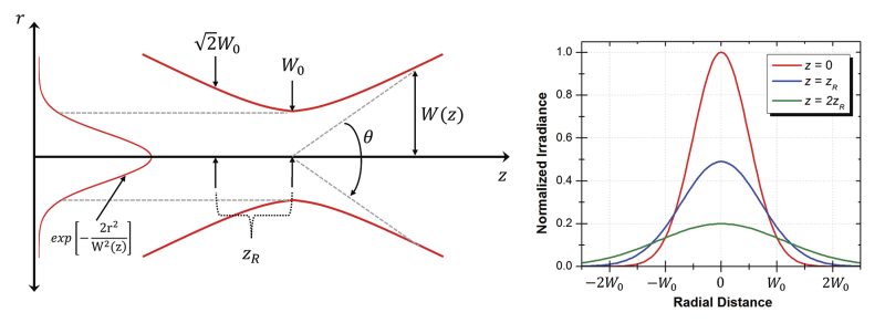
The equation describing the evolution of the beam radius along the axis where z is the distance from the beam waist is given by:

zR is known as the Rayleigh range and represents the distance from the waist where the radius increases by a factor of . If above equation is substituted into irradiance distribution equation, then zR is the distance at which the irradiance has decreased by a factor of √2 from its peak value at the waist. Twice the Rayleigh range is called the confocal parameter (or depth-of-focus) and is a rough estimate of the collimation of a beam. As shown in the above equation, the beam size increases slowly with axial distance from the waist. As z >> zR, the beam size then increases linearly with z with a slope of W₀/z_R. This slope represents the full angular width divergence (θ) of the beam given by:

A clear reciprocal relationship exists between the spot size (2W₀) and the divergence. In addition, for a Gaussian beam at a given wavelength, the product of the spot size and the divergence is a constant at 4λ/π. This is important in defining how much a beam deviates from a perfect Gaussian beam.

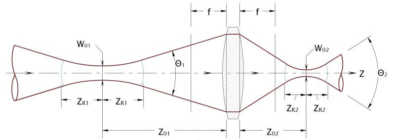
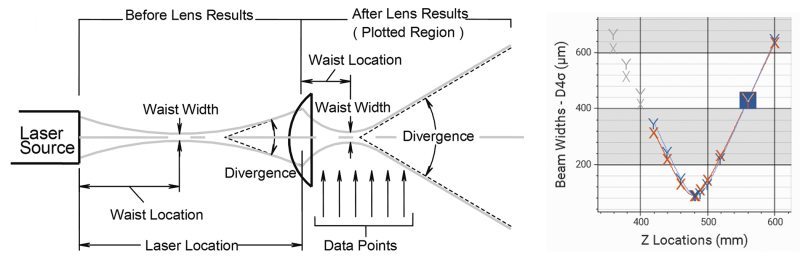
Laser beams are often propagated through an optical system consisting of lenses, mirrors, dielectric interfaces, or other optical elements. Fortunately, under most conditions, a Gaussian beam remains a Gaussian beam after encountering these elements, ensuring that the propagation equations used above remain valid. An optical element modifies the input beam by changing the position and size of its beam waist. Knowledge of the input beam parameters and the properties of the optical element can be used to determine the new values using a variety of propagation methods. A thin focusing lens  is probably the most important optical element that impacts a laser beam. Figure 2 illustrates beam propagation through a thin lens resulting in a repositioning and resizing of the beam waist (as well as z_R and θ). When a collimated beam (i.e., 2.zR >> f) encounters a lens, the resulting beam waist is simply the product of the focal length and original divergence (see full angular width divergence equation) with the waist positioned at the focal point of the lens.

The TEM₀₀ mode of even a well-designed laser system is not a perfect Gaussian beam. The M² ("M-Squared") analysis was developed to characterize the quality of a laser beam. That is, how close it is to an ideal Gaussian beam. M² is defined as the product of the spot size (2W_M) and divergence (θ_M) of the real beam divided by the spot-size-divergence product of an ideal Gaussian beam:

One practical consequence of this definition is that an ideal Gaussian beam (i.e., M² = 1) can be focused to a minimum spot diameter, whereas beams of higher M. values focus to larger spot diameters in proportion to the M² value. As a result, M² provides meaningful information about lasers, particularly if their application involves small focused spot sizes. While W_M and θ_M are sufficient for determining M², these values often cannot be measured directly. By focusing the beam with a lens of known focal length (like Figure 2), the characteristics of the artificially created beam waist and divergence can be measured. To provide an accurate calculation of M², the International Organization for Standards (ISO) requires at least 5 measurements in the focused beam waist region and at least 5 measurements in the far fields (two Rayleigh ranges away from the waist area), as shown in Figure 3. These multiple measurements ensure that the minimum beam width is found while a "curve fit" improves the accuracy by minimizing measurement error at any single point.

A commonly-available helium-neon laser emits a near-ideal Gaussian beam with a value of M² < 1.1. For many solid-state lasers, M. is in the range of 1.1-1.3. Collimated laser diodes that emit fundamental TEM₀₀ modes possess M. of 1.1 to 1.7, whereas high-energy multimode lasers can generate M² factors as large as 10 to 100. Spatial filtering can improve beam quality using Fourier optics. Finally, additional beam quality metrics include the Beam Propagation Factor (K) where K = 1/M² as well as the Beam Parameter Product (BPP), which is defined as BPP = M²λ/π = 2W_M.M²

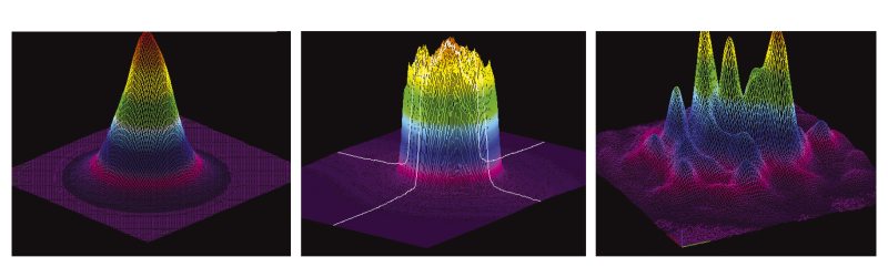
While many laser systems operate with near-Gaussian beams, other laser systems possess non-Gaussian beams that propagate differently and exhibit significantly different spatial distributions (see Figure 4 for examples). In some cases, a laser resonator emits a beam with a higher-order TEM_mn mode. Depending on the resonator geometry, these modes can be cylindrical in nature and are called Laguerre-Gaussian beams or rectangular and are called Hermite-Gaussian beams. In other cases, a laser beam is modified by an optical system to such an extent that its profile and propagation can no longer be approximated using the Gaussian beam analysis. Flat-top beams are one such example where a beam exhibits a nearly constant irradiance over its beam width (see Figure 4). Given the steep edges of the beam profile, the diameters of these beams are often characterized by their full-width at half-maximum (FWHM) values as opposed to the HW1/e² radius values used for Gaussian beams. Such flat-top beams are important for laser-based material processing where a constant irradiance provides more uniform material modification. The propagation of these beams can be quite complicated and is often encountered when a laser beam overfills a focusing objective in order to generate a very small spot size in high-resolution microscopy.